
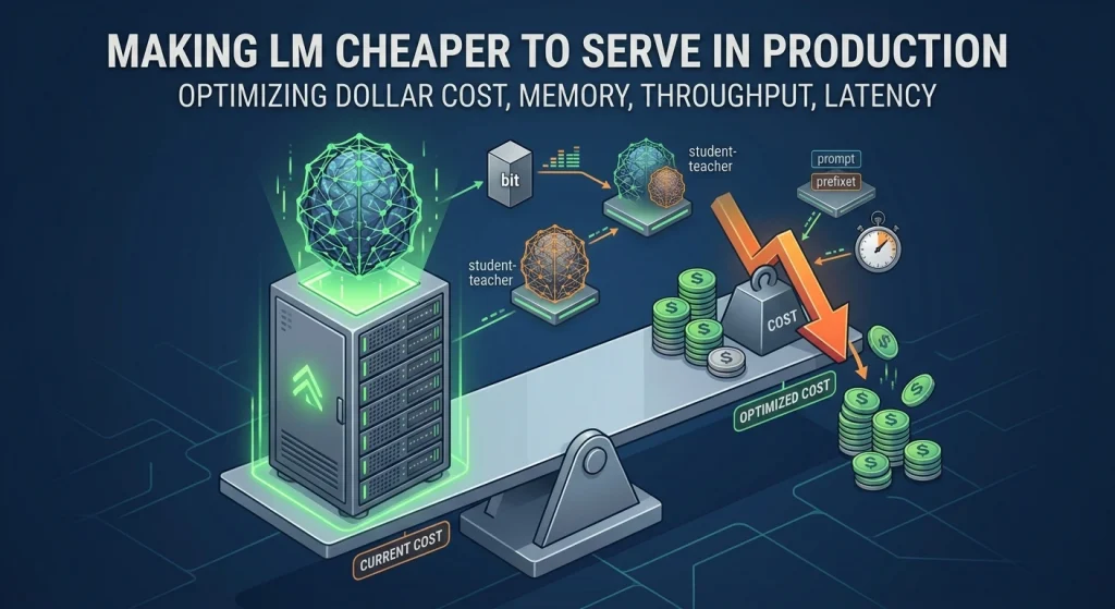
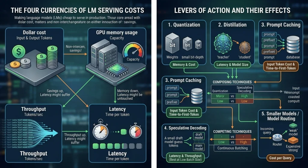
Serving a language model costs money in four distinct currencies — input and output tokens billed in dollars, GPU memory, throughput (tokens per second), and latency (time to first token and time per token). A savings figure is meaningless unless it names which of those it is measured in, and the techniques below are not interchangeable between them: the same method that halves memory can leave latency untouched, and a change that raises throughput can leave latency per query worse. The five levers named in the question — quantization, distillation, prompt caching, speculative decoding, and smaller or routed models — and a sixth group of serving-time levers (continuous batching, KV-cache management, pruning, and batch APIs) are covered below: how each works, what published measurements report, and the boundary conditions under which the reported gains shrink.
1. Quantization
Quantization stores a model’s numbers in fewer bits than the 16-bit floating point they are trained in. The engineering splits into three axes:
- What gets quantized — weights only, or weights and activations, or the KV cache.
- How reduced-precision values are recovered — calibration, scaling, or mixed-precision fallback.
- Whether dedicated kernels exist — to realize a wall-clock gain rather than only a memory gain.
Weight-only, 4-bit. GPTQ quantizes a pretrained model layer by layer against a small calibration set, and reports 3–4 bits per weight in roughly four GPU-hours on a single A100, with negligible perplexity degradation [1]. On OPT-175B, 4-bit GPTQ costs only +0.03 WikiText2 perplexity against the FP16 baseline. Round-to-nearest quantization at the same width, by contrast, loses 2.2 points — worse than a full-precision model ten times smaller — and collapses entirely at 3 bits. With custom kernels the 3-bit model fits in roughly 63 GB (one 80 GB A100, against five for FP16) and runs at about 3.25x lower per-token latency (71 ms vs 230 ms). The authors are explicit that the speedup comes from reduced memory movement, not fewer FLOPs.
AWQ attacks the same problem from the accuracy side: it observes that only about 0.1–1% of weight channels are salient, identifies them by activation magnitude rather than weight magnitude, and protects them by per-channel scaling rather than by mixed-precision storage [2]. Scaling the salient channels lifts OPT-6.7B INT3 WikiText2 perplexity from 23.54 to 11.92, close to the 13.0 obtained by keeping 1% of weights in FP16 — without the hardware cost of mixed-precision math. The companion engine, TinyChat, reports a 3.2–3.3x average speedup over HuggingFace FP16, up to 3.9x on an RTX 4090.
Weight and activation, 8-bit. LLM.int8() quantizes both weights and activations but isolates the large-magnitude “outlier” feature dimensions that emerge around 6.7B parameters (about 0.1% of dimensions) into a 16-bit path, cutting inference memory roughly in half up to 175B parameters while retaining full-precision performance [3]. Its speed story is conditional and important: raw INT8 matmul beats FP16 only at large model dimensions. Once quantization and outlier-decomposition overhead are counted, LLM.int8() is a net slowdown below a model dimension of roughly 4096–5140 and speeds up only the 13B and 175B sizes. In end-to-end BLOOM-176B generation it is roughly on par with bfloat16 per token, but lets the model fit on fewer GPUs.
SmoothQuant removes the outlier problem by mathematically migrating activation difficulty into the weights, enabling full W8A8 quantization [4]. Naive per-tensor W8A8 collapses OPT-175B to 0.0% LAMBADA accuracy and a WikiText2 perplexity of 93080 — effectively random. SmoothQuant, by contrast, preserves near-FP16 accuracy and reports up to 1.56x speedup with 2x memory reduction, enough to serve the 530B MT-NLG model on a single 8-GPU node for the first time. ZeroQuant takes a similar W8A8 route with group-wise weight and token-wise activation schemes plus an optional layer-wise distillation step, and explicitly criticizes prior work for reporting only theoretical compression: measured on A100s it reaches up to 5.19x speedup on BERT-base and, on GPT-J-6B, 3.67x speedup, cutting the GPU requirement from two A100s to one and latency from 65 ms to 25 ms [5].
KV-cache quantization. The cache, not the weights, becomes the dominant memory consumer at scale — for PaLM-540B at batch 512 and 2048-token context the KV cache alone reaches 3 TB, three times the model’s parameters [6]. KIVI quantizes it to 2 bits asymmetrically, per-channel for keys and per-token for values, on the empirical finding that keys carry channel-wise outliers while values do not [7]. It reports 2.6x peak-memory reduction for Llama-2-7B (weights included) with up to a 2% accuracy drop, and because the freed memory allows larger batches, 2.35–3.47x higher throughput on a single A100 — a gain that grows with context length.
What the savings cost. The strongest independent caution is that aggregate benchmark accuracy hides behavioral divergence: across six quantization schemes, accuracy moved by at most 2%, while up to 13.6% of individual answers flipped between correct and incorrect. Only GPTQ W8A16 showed negligible flips [8]. The damage is structured rather than uniform. At 8 bits the average long-context drop is about 0.8%, but 4-bit methods lose up to 59% on specific long-context retrieval tasks, worsening as context grows [9]. Multilingually, automatic metrics understate the harm badly — a 1.7% automatic drop in Japanese corresponds to a 16.0% drop under human evaluation of realistic prompts — and non-Latin-script and lower-resource languages degrade fastest [10]. A large-scale study of over 500,000 evaluations on the Llama-3.1 family finds FP8 effectively lossless, INT8 with a surprisingly low 1–3% degradation, and INT4 weight-only rivaling 8-bit, reporting 2–3x lower cost per query for 8B/70B and 5–7x at 405B [11]. The reconciliation is that quantization’s cost is workload-shaped: it is cheapest to defend on large models, short English contexts, and easy tasks, and most expensive on long-context, multilingual, or reasoning-heavy work.
2. Distillation
Distillation trains a small “student” model to reproduce a larger “teacher.” The foundational formulation transfers the teacher’s temperature-raised softmax outputs as soft targets, which carry more information per example than hard labels and act as a strong regularizer [12]. On MNIST, matching a large regularized teacher’s soft targets halves the error of an identically sized hard-label model (74 vs 146 test errors). Distilling a ten-model ensemble into a single 85M-parameter acoustic model recovers more than 80% of the ensemble’s frame-accuracy gain while matching its word-error rate.
The modern encoder example is DistilBERT, which distills during pretraining with a triple loss (soft-target cross-entropy, masked-language-modeling, and a cosine hidden-state alignment term), yielding a model 40% smaller (66M vs 110M parameters) and 60% faster on CPU while retaining 97% of BERT-base’s GLUE score [13]. On-device it is 71% faster for question answering on an iPhone 7 Plus at a 207 MB model size.
For large language models two variants matter. Distilling step-by-step has the teacher emit a chain-of-thought rationale alongside each label and trains the student to predict both, so the reasoning is used as training signal but never needed at inference [14]. A 770M T5 student then outperforms a few-shot 540B PaLM on natural-language inference using only 80% of the labeled data, and across four benchmarks the method reaches better accuracy than standard fine-tuning with over 50% fewer examples on average. Minitron combines structured pruning of a pretrained model with distillation-based retraining to derive a whole family of smaller models from one large one: deriving 8B and 4B models from a 15B teacher uses up to 40x fewer training tokens per model and saves 1.8x training compute for the family, with the 8B model matching Mistral 7B and Llama-3 8B on MMLU despite training on only 94B tokens [15].
The boundary condition is the source of the teacher’s signal. Distillation proper assumes white-box access to a teacher whose data, architecture, and probability distribution are known; imitating a proprietary API from its text outputs is a harder, black-box problem. Imitation models trained on up to 150M tokens of a commercial assistant’s outputs are rated equal-or-better by about 70% of crowdworkers yet fail to improve — and sometimes regress — on MMLU, Natural Questions, and HumanEval, because they imitate confident tone and formatting rather than factual accuracy [16]. Task-specific imitation closes much more of the gap than broad imitation, and scaling the base model beats scaling the imitation data.
3. Prompt Caching
Prompt caching reuses the attention state (the KV cache) of a prefix the model has already processed, so a shared system prompt, tool definition, or document is billed and computed once rather than on every call. It appears in two forms: provider-side API caching and server-side cache reuse inside a serving engine.
Provider APIs. The three major providers price cached input differently:
| Provider | Cache write | Cache read | Minimum cached prefix | Default TTL |
|---|---|---|---|---|
| Anthropic | 1.25x base input [17] | 0.1x (0.05x Opus 5.5; 0.025x Fable 5.1 / Mythos 5.1) [17] | — | 5 min, refreshed on each hit; 1-hour option |
| OpenAI | — | flat 50% discount on cached input | above 1,024 tokens, in 128-token increments [18] | cleared after 5–10 min of inactivity |
| — (implicit, on by default) | automatic pass-through | 2,048 tokens for 2.5 Flash/Pro; 4,096 for newer [19] | — |
Anthropic’s own launch benchmarks report up to 90% cost reduction and up to 85% latency reduction on long prompts, with a 100,000-token “chat with a book” workload dropping time-to-first-token from 11.5 s to 2.4 s [20].
Independent measurement. A controlled study across OpenAI, Anthropic, and Google found prompt caching cuts API cost by 41–80% and improves time-to-first-token by 13–31% on a long-horizon agentic workload [21]. The best result was GPT-5.2 at 79.6% cost reduction; Claude Sonnet 4.5 reached 78.5% cost reduction with the largest TTFT gain of 22.9%; Gemini 2.5 Pro was lowest at 41.4% and 6.1%. The study shows the strategy matters more than the feature: caching dynamic tool-call results (“full-context” caching) can paradoxically increase latency, with GPT-4o regressing 8.8% on TTFT, and the reliable recipe is to keep dynamic content out of the cached region and place it at the end of the prompt.
Server-side reuse. SGLang’s RadixAttention keeps KV cache across requests in a radix tree with LRU eviction, rather than discarding it when a generation ends, and reports up to 6.4x higher throughput and 3.7x lower latency than vLLM and other engines [22]. In a one-month production deployment on LMSYS Chatbot Arena it sustained cache hit rates of 52.4% and 74.1% — demonstrating that the theoretical reuse is realized under real traffic. A separate system, Prompt Cache, precomputes attention states for schema-defined reusable segments and reports 8–10x time-to-first-token reduction on GPU and 20–70x on CPU [23].
Conditions and risks. Caching requires an exact prefix match up to the breakpoint — any change to content at or before it, to tool-use settings, or even to JSON key ordering in some SDKs breaks the cache [17]. Because savings scale with how much of the prompt is reusable, caching pays off in exactly the workloads with large, stable prefixes (long system prompts, few-shot exemplars, document QA, multi-turn agents) and pays little where prompts are short or highly variable. A privacy caution also attaches to it: a timing audit detected prompt caching in 8 of 17 API providers and global cross-user cache sharing in 7, inferring which prompts other users had sent from response timing [24].
4. Speculative Decoding
Autoregressive decoding is memory-bandwidth bound — generating one token reads the whole model’s weights for a single output. Speculative decoding exploits the resulting spare compute: a small draft model proposes several tokens, the large target model scores all of them in one parallel forward pass, and a rejection-sampling rule accepts the longest valid prefix. The standard scheme is provably lossless, producing output distributed identically to sampling from the target model alone. Because it does not modify the target model, it composes with quantization [25] [26].
The scheme’s benefit is governed by the acceptance rate — the fraction of drafted tokens the target accepts — and by the context. Leviathan et al. report 3.4x speedup (greedy) on English–German translation with an 11B target and a 77M draft, and note that even a trivial bigram drafter with a 0.2 acceptance rate yields 1.25x [25]. Chen et al. report 1.92–2.46x on a 70B target with a purpose-trained 4B draft, with higher acceptance on code than on summarization because code contains more predictable sub-sequences [26]. The idea is older than the term: blockwise parallel decoding used trained prediction heads four years earlier to double greedy decoding speed at no quality loss [27].
Later variants remove or reduce the need for a separate draft model. Medusa adds lightweight feed-forward heads that predict several positions at once and verifies tree-shaped candidates, reporting 2.2–2.8x on Vicuna [28]. EAGLE drafts at the feature level rather than the token level and reports 2.7–3.5x and doubled throughput on a 70B target [29]. SpecInfer organizes candidates from several small models into a token tree and verifies it in one pass, raising per-token acceptance from 52–57% to 96–97% and reaching 1.5–2.8x for distributed serving and 2.6–3.5x for single-GPU offloading [30]. A third-party benchmark of six task types found EAGLE the strongest of the compared methods at 1.8–2.4x [31].
The boundary conditions are where the savings erode. Speedup falls as sampling temperature rises — EAGLE drops from 2.08x at T=0 to 1.74x at T=1.0 — because higher-entropy targets make verification stricter [31]. It falls as batch size rises, because batching consumes the spare compute speculation needs: EAGLE declines from 2.90x to 2.65x on a 7B model and from 3.01x to 2.40x on a 70B model between batch 1 and batch 4 [29]. The optimal draft length shrinks with batch size (about k=4–5 at batch 1 versus k=1–2 at batch 64), and at high batch size with a middling acceptance rate speculation can invert into a net slowdown below 1.0x — which is why a goodput-aware controller that disables speculation when it would hurt is worth having [32]. On mixture-of-experts models the gain collapses toward 1.5x because verifying several tokens touches more experts per step and erodes the sparse-compute advantage. And the technique only helps when the target is memory-bound with spare compute available; where compute is the constraint, it is not helpful at all [25].
5. Smaller Models and Model Routing
The cheapest token is the one a large model never has to produce, and there are two distinct ways to arrange that: choose a smaller model that is good enough, or route each query to the cheapest model that can handle it.
Right-sizing. The Chinchilla scaling laws showed that for a fixed training budget, model size and training tokens should scale equally. The authors validated this by training a 70B model on 1.4T tokens that outperformed 175B, 178B, 280B, and 530B contemporaries while reaching a then-state-of-the-art 67.5% on MMLU [33]. The paper notes the smaller model also cuts inference cost, but its objective is training-time compute only. Inference-aware scaling makes the point sharper: once expected inference volume is priced in, the optimal model is smaller and trained longer, so a developer expecting two trillion inference tokens can cut total compute 17% by training a 7B model instead of a 13B one, and in dollar terms — because inference runs at far lower hardware utilization than training — a Chinchilla-70B model costs 36% more than a cost-optimal model of equal quality [34]. This reframes the whole levers list: how much a model will be served, not only how good it is, determines how large it should be.
Cascades and routing. FrugalGPT queries cheap APIs first and escalates to expensive ones only until a learned reliability score passes a threshold. It matches GPT-4’s accuracy at up to 98% lower cost and saves 59.2–98.3% across finance, legal, and reading-comprehension datasets [35]. RouteLLM trains a binary router on preference data to send each query to a strong or weak model under a cost threshold, reducing cost by over 2x while retaining quality, and up to 3.66x with 95% of GPT-4’s MT-Bench score [36]. Both make the same structural point: commercial model prices differ by up to two orders of magnitude, so the choice of which model answers a query dwarfs most per-token optimizations. Hybrid LLM routes each query to exactly one model and reports 40% fewer large-model calls at no quality drop, with the router itself running about 10x faster than the fastest model it dispatches to [37].
Conditions. Routing assumes a quality signal that generalizes: routers trained only on one model pair still transfer to unseen pairs (RouteLLM reports 30–55% improvements over random on new Claude and Llama pairs), but the gains track how closely the new pair’s quality gap resembles the training pair’s [36] [37]. Cascades and routers also need labeled examples resembling the traffic and carry a one-time cost to learn, and their overhead is small but nonzero (RouteLLM’s most expensive router adds no more than 0.4% of GPT-4’s generation cost).
6. Other Production Levers
Several levers outside the five named techniques move cost as much as anything above.
Continuous batching and memory management. Orca introduced iteration-level scheduling — deciding the batch one decode step at a time, so finished requests leave and new ones join immediately. It reported 36.9x higher throughput than FasterTransformer at matched latency on GPT-3 175B [38]. vLLM’s PagedAttention then treats the KV cache as non-contiguous fixed-size blocks, raising effective cache utilization from the 20.4–38.2% observed in earlier systems to 96.3% and enabling 2–4x higher request rates (up to 22x over FasterTransformer) [39]. These are throughput levers, and they carry the field’s central tradeoff: smaller batches give lower latency but worse hardware utilization and higher cost per token, while large batches minimize cost per token but worsen latency — one configuration cannot be both latency-optimal and cost-optimal [6].
Pruning and sparsity. SparseGPT prunes GPT-scale models to 50–60% sparsity in one shot with no retraining and negligible accuracy loss, in under 4.5 hours on a single A100 — and finds larger models more compressible, with the perplexity loss at 50% sparsity shrinking to near zero at 66B and 175B parameters [40]. It also composes with quantization: 50% sparsity plus 4-bit quantization beats a size-equivalent pure 3-bit model.
KV-cache compression. The KV cache can exceed the weights by 3x at large batch and long context [6], compressing it (for example KIVI’s 2-bit scheme) raises the batch size the hardware can sustain and therefore throughput [7]. Multiquery attention makes the same trade on the architecture side, sharing one key/value head across all query heads to enable up to 32x longer contexts at equal memory [6].
Batch APIs. All three major providers offer a flat 50% discount for asynchronous bulk workloads with a 24-hour turnaround target [41] [42] [43]. This is the simplest lever on the list — no model change, no accuracy cost — but it applies only to non-latency-sensitive work, and each provider imposes caps (Anthropic at 100,000 requests or 256 MB per batch). Batching also interacts with other levers: Gemini charges cache-hit requests inside a batch at the cache rate so the two stack, while Anthropic does not support cache pre-warming inside a batch because the ephemeral cache entry would expire before a follow-up request runs [42].
7. Comparing and Combining the Techniques
The techniques cannot be ranked on a single axis, because they save different currencies:
| Technique | What it saves | Representative measured figure | Main condition / cost |
|---|---|---|---|
| Quantization (weight-only) | Memory, cost per query | GPTQ 4-bit: +0.03 PPL on OPT-175B; 3.25x per-token latency; W4A16 2–3x cost/query (8B–70B), 5–7x (405B) [1] [11] | Accuracy loss grows on long-context, multilingual, reasoning tasks |
| Quantization (KV cache) | Memory, throughput | KIVI 2-bit: 2.6x peak memory, 2.35–3.47x throughput [7] | Up to ~2% accuracy drop; implementation overhead unfused |
| Distillation | Model size, latency | DistilBERT 40% smaller, 60% faster, 97% retained [13]; step-by-step 770M T5 beats 540B PaLM [14] | Requires a teacher; broad black-box imitation largely fails |
| Prompt caching | Input-token cost, TTFT | 41–80% cost, 13–31% TTFT across three providers [21] | Needs a large stable prefix; cache breaks on any prefix change |
| Speculative decoding | Latency, throughput | 2–3.5x at batch 1 (EAGLE, Medusa, SpS) [30] [29] | Shrinks with batch size, temperature, MoE; needs spare compute |
| Smaller / routed models | Cost per query | Cascades up to 98% cost reduction [35]; RouteLLM 3.66x [36] | Needs a quality signal that generalizes; one-time learning cost |
| Continuous batching / PagedAttention | Throughput | vLLM 2–4x request rate, up to 22x vs FasterTransformer [39] | Throughput-latency tradeoff; batch-size ceiling |
| Batch APIs | Cost | Flat 50% discount [41] | Non-latency-sensitive workloads only |
Do the savings stack? Partly, and the pattern is that techniques operating on different resources compose, while techniques competing for the same resource compete. Quantization and speculative decoding compose cleanly: speculation does not modify the target model’s weights, so it can be layered over quantized inference, and Medusa’s and EAGLE’s best published numbers come from combining speculative heads with 4-bit kernels [26] [29]. Pruning and quantization also compose, with 50% sparsity plus 4-bit beating size-equivalent 3-bit [40]. Caching and batching compose at the billing layer where the provider permits it [43]. But two throughput-hungry techniques do not stack: speculative decoding and continuous batching draw on the same spare compute, which is why speculation’s speedup decays as batch size grows and can go negative [32].
Which lever dominates depends on the workload, not the technique. For cost-per-query on API-served models, routing and cascades report the largest reductions (up to 98%) because they exploit the two-orders-of-magnitude spread in model prices, with prompt caching second (41–90% on the cached fraction of input). For self-hosted serving, quantization is the broadest memory-and-cost lever and is essentially mandatory at the large end — the 405B case runs at 5–7x lower cost and on a quarter of the GPUs — while batching and PagedAttention set the throughput ceiling. Speculative decoding is a latency lever that pays only when the target is memory-bound and batches are small; its benefit is the most fragile of any technique here. The consistent lesson across all of them is to state the metric and the conditions. Nearly every headline figure in this report was measured at batch size 1, on short English prompts, at low temperature, or under a specific provider’s cache policy. The same technique measured outside those conditions often reports a fraction of the saving — or, in the case of full-context caching, a regression.
Sources
- Elias Frantar et al. (2022). GPTQ: Accurate Post-Training Quantization for Generative Pre-trained Transformers. arXiv.org. arXiv:2210.17323 [1]
- Ji Lin et al. (2023). AWQ: Activation-aware Weight Quantization for On-Device LLM Compression and Acceleration. Conference on Machine Learning and Systems. arXiv:2306.00978 [2]
- Tim Dettmers et al. (2022). LLM.int8(): 8-bit Matrix Multiplication for Transformers at Scale. Advances in Neural Information Processing Systems 35. arXiv:2208.07339 [3]
- Guang-Xuan Xiao et al. (2022). SmoothQuant: Accurate and Efficient Post-Training Quantization for Large Language Models. International Conference on Machine Learning. arXiv:2211.10438 [4]
- Z. Yao et al. (2022). ZeroQuant: Efficient and Affordable Post-Training Quantization for Large-Scale Transformers. Neural Information Processing Systems. arXiv:2206.01861 [5]
- EFFICIENTLY SCALING TRANSFORMER INFERENCE. arXiv:2211.05102 [6]
- KIVI: A Tuning-Free Asymmetric 2bit Quantization for KV Cache. arXiv:2402.02750 [7]
- Accuracy is Not All You Need. arXiv:2407.09141 [8]
- Anmol Reddy Mekala et al. (2025). Does quantization affect models’ performance on long-context tasks?. Conference on Empirical Methods in Natural Language Processing. arXiv:2505.20276 [9]
- Kelly Marchisio et al. (2024). How Does Quantization Affect Multilingual LLMs?. Conference on Empirical Methods in Natural Language Processing. arXiv:2407.03211 [10]
- “Give Me BF16 or Give Me Death”?. arXiv:2411.02355 [11]
- Geoffrey E. Hinton et al. (2015). Distilling the Knowledge in a Neural Network. arXiv.org. arXiv:1503.02531 [12]
- Victor Sanh et al. (2019). DistilBERT, a distilled version of BERT: smaller, faster, cheaper and lighter. arXiv.org. arXiv:1910.01108 [13]
- Cheng-Yu Hsieh et al. (2023). Distilling Step-by-Step! Outperforming Larger Language Models with Less Training Data and Smaller Model Sizes. Annual Meeting of the Association for Computational Linguistics. arXiv:2305.02301 [14]
- Compact Language Models via Pruning and. arXiv:2407.14679 [15]
- Arnav Gudibande et al. (2023). The False Promise of Imitating Proprietary LLMs. arXiv.org. arXiv:2305.15717 [16]
- Prompt caching – Claude Platform Docs. https://docs.claude.com/en/docs/build-with-claude/prompt-caching [17]
- Prompt Caching in the API | OpenAI. https://openai.com/index/api-prompt-caching/ [18]
- Context caching | Gemini API | Google AI for Developers. https://ai.google.dev/gemini-api/docs/caching [19]
- Prompt caching with Claude | Claude by Anthropic. https://www.anthropic.com/news/prompt-caching [20]
- Elias Lumer et al. (2026). Don’t Break the Cache: An Evaluation of Prompt Caching for Long-Horizon Agentic Tasks. arXiv.org. arXiv:2601.06007 [21]
- SGLang: Efficient Execution of. arXiv:2312.07104 [22]
- PROMPT CACHE: MODULAR ATTENTION REUSE. arXiv:2311.04934 [23]
- Chenchen Gu et al. (2025). Auditing Prompt Caching in Language Model APIs. International Conference on Machine Learning. arXiv:2502.07776 [24]
- Fast Inference from Transformers via Speculative Decoding. arXiv:2211.17192 [25]
- Accelerating Large Language Model Decoding. arXiv:2302.01318 [26]
- Mitchell Stern et al. (2018). Blockwise Parallel Decoding for Deep Autoregressive Models. Neural Information Processing Systems. arXiv:1811.03115 [27]
- MEDUSA: Simple LLM Inference Acceleration Framework with Multiple. arXiv:2401.10774 [28]
- Yuhui Li et al. (2024). EAGLE: Speculative Sampling Requires Rethinking Feature Uncertainty. International Conference on Machine Learning. arXiv:2401.15077 [29]
- SpecInfer: Accelerating Large Language Model Serving. arXiv:2305.09781 [30]
- Heming Xia et al. (2024). Unlocking Efficiency in Large Language Model Inference: A Comprehensive Survey of Speculative Decoding. Annual Meeting of the Association for Computational Linguistics. arXiv:2401.07851 [31]
- Xiaoxuan Liu et al. (2024). TurboSpec: Closed-loop Speculation Control System for Optimizing LLM Serving Goodput. arXiv:2406.14066 [32]
- Training Compute-Optimal Large Language Models. arXiv:2203.15556 [33]
- Nikhil Sardana et al. (2023). Beyond Chinchilla-Optimal: Accounting for Inference in Language Model Scaling Laws. International Conference on Machine Learning. arXiv:2401.00448 [34]
- FrugalGPT: How to Use Large Language Models. arXiv:2305.05176 [35]
- Published as a conference paper at ICLR 2025. arXiv:2406.18665 [36]
- Hybrid LLM: Cost-Efficient and Quality-Aware Query Routing. arXiv:2404.14618 [37]
- This paper is included in the Proceedings of the. https://www.usenix.org/system/files/osdi22-yu.pdf [38]
- Efficient Memory Management for Large Language. arXiv:2309.06180 [39]
- Elias Frantar and Dan Alistarh (2023). SparseGPT: Massive Language Models Can Be Accurately Pruned in One-Shot. International Conference on Machine Learning. arXiv:2301.00774 [40]
- Batch API | OpenAI API. https://platform.openai.com/docs/guides/batch [41]
- Batch processing – Claude Platform Docs. https://docs.claude.com/en/docs/build-with-claude/batch-processing [42]
- Batch API | Gemini API | Google AI for Developers. https://ai.google.dev/gemini-api/docs/batch-mode [43]
This article includes content created with AI.